Rose Mary, she likes berries, believes in Fairies and is in love with Harry

We will explain here, how to carry out the Harris Corner Detector Algorithm in Matlab.
We will divide the task in 2 parts, one part will calculate the corner points of the image, and the other part, will draw small squares around those corner points with the purpose of having a way of displying them to the user.
The part of detecting the corner points of the image is the following:

%we create a function named harris that receives an rgb image
%and the desired k value. We will return a matrix named A that
%has information about whether or not a certain pixel represents
%a corner.
function [A] = harris(rgb, k)


%If we received an RGB image we convert it to Gray Scale.
%We do this, because if we were to work with an RGB image it
%would be necessary to work with 3 channels, the red, green and blue channel, %instead of just one, which is possible with the gray scale image .

if( size(rgb,3) >= 3 )
img = double( rgb2gray(rgb) );
end

%Before , we continue , it is important to recall that in the Harris Corner Detector, %we obtained a weighted sum of squared differences between an area (uv) and %another area that was obtained by shifting the original area by (x,y), and thus we %had the following form:

%w(u,v) represented a weighted sum. It is important to note that I(u + x,v + y) %can be approximated by a Taylor expansion.

%Where Ix and Iy are the partial derivatives of I.
%Resulting in:

%Since we will carry out an operation that involves partial derivatives we need to %carry out a smoothing, because computation of derivatives generally involves a %stage of scale-space smoothing. For this,we will use the convolution of the gray %image with a Gaussian kernel.
So the next steps that we will carry out are:
a) Calculate the partial derivatives with respect to X and to respect to Y of the image. This will give us the gradients with respect to X and with respect to Y.
b) convolve these gradients with a Gaussian Kernel.
The following is our Gaussian Kernel, which will give us blurring on both directions%

g = 1/16 * [1 2 1; 2 4 2; 1 2 1];

%Here we define the Gradients Operators, we will use the Prewitt Gradient Kernel to obtain the gradients. If we pay more attention to this matrix, we notice that this kernel considers that the orthogonal and diagonal pixel differentials equally

dx = [-1 0 1; -1 0 1; -1 0 1]; %Prewitt Gradient Kernel in X
dy = dx';

% We obtain all the partial derivatives in x and y of the image. These are the %Gradient values.
Ix = conv2(img, dx, 'same');
Iy = conv2(img, dy, 'same');
% We obtain a matrix, that will have the product of Ix*Iy for all Ix and all Iy
Ixy= Ix .* Iy;

% We will now obtain the square value of Ix and of Iy and we will obtain a blurring of Ix square,Iy square and of Ixy.The blurring will be carried out by using the gaussian kernel.We need those square values , since let's recall we had the following:

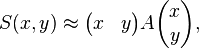
Which produces the approximation

which can be written in matrix form:

where A is:

%So we calculate the values that are inside this matrix.

Ix2 = conv2(Ix .* Ix, g, 'same');
Iy2 = conv2(Iy .* Iy, g, 'same');
Ixy = conv2(Ixy, g, 'same');


%We now have 3 matrices , Ix2 that hold the values of all the xs in the image, but they are squared and have been convolved with a Gaussian, so all the xto the square values are blurred a bit. It is important to note, that this operation helps to reduce noise. It smooths the image. We have another matrix Iy2 with the ys to the square value and also blurred as well as third matrix Ixy that holds the values of all the x's times their corresponding y. All 3 of these matrices will help us to calculate the Harris corner response that each pixel of the image has.
The Harris Corner response for each pixel will come out of a matrix A, that as we had said before handwas conformed of:

%Where Ix represents the x value of the pixel, and Iy the y value of the pixel. The Harris Corner response %of a pixel will be Mc:

%What our Harris Function will return will be a matrix that will hold the harris corner response for each %one of the pixels that conform the image:

A = (Ix2.*Iy2 - Ixy.^2) - k * (Ix2 + Iy2).^2;

end

We will now write the function that draws a small red square around the detected corner points.

%This function receives the image we wish to detect and draw the corner points of, %it also receives the desired k value to use, and the desired threshold. It is %important to remember that in the Harris corner detector, we consider a corner %to be a corner when the measure of corner response surpasses a certain %threshold. This measure is computed through the determinant and the trace of the % matrix.

function img_h = project1(img, k, threshold)
%We store the original image in img_h, we need to store it, since we will draw the %squares denoting the corners above it.
img_h = img;
%We use the function we had defined above and with it obtain a matrix that holds %all the corner response measures for all the pixels of the image%
M = my_harris(img, k);

%We iterate through the whole matrix
for x = 2 : size( M, 1 )
for y = 2 : size(M, 2)
%If we find a point of the matrix, that has a value above the threshold, then that %point is a corner and we will draw a rectangle on that pixel.
if M(x,y) > threshold
for xpos = x - 1:x+1
img_h(xpos,y-1,1) = 255;
img_h(xpos,y+1,1) = 255;
end

for ypos = y - 1:y+1
img_h(x-1,ypos,1) = 255;
img_h(x+1,ypos,1) = 255;
end
end
end
end

end

We now present a image that was used for this purpose.
The original image is:

And the image with the corners detected is: